Have you ever held an abacus in your hands? Chances are yes. Many grade schools use this ancient calculating device as a way of introducing students to some fundamental aspects of mathematics.

Have you ever held a slide rule in your hands? If you are a so-called “millennial” or slightly older, chances are not. Why? Because the slide rule, which in its day was considered by many as the eighth wonder of the world, has virtually passed away without a trace.

I grew up when slide rules were very much at the height of their powers (the 1940s and 1950s). Although I fully understand why the slide rule seems to have sunk out of sight, I mourn its passing. This is not just nostalgia. When affordable electronic calculators were introduced in the 1970s, I was one of the first to sing their praises as an ineffable advance over the slide rule. However, there was a problem. I had no idea how an electronic calculator worked. By contrast, because it was based on a very simple but far-reaching mathematical principle, I did understand how the slide rule worked. I could have even built one myself!

The fundamental premise of this blog series “Extraordinary Ordinary Things” is to explore truly historic things that have become so integral to our lives we seldom notice them and hardly ever think about them. As a kind of departure from this general theme, I would like to take a fond look back at the slide rule and what it meant to those of us who grew up with it and used it during its heyday.

For engineers in the ‘40s,’ 50s, and ‘60s, the slide rule was as inconspicuous as the other extraordinary ordinary things we have discussed. Today it is still inconspicuous—because it has largely disappeared.

The Principle

The slide rule is founded on the principle of logarithms. By the simplest definition, a logarithm is an exponent, i.e. it is the power to which a number must be raised to give a specified result. This can be done in any number base, but the easiest one to understand is base 10, because this is what the decimal number system we use every day is all about.

For example, in base 10, the logarithm of 10 itself is 1 because 10 x 1 = 10¹ = 10; the logarthm of 100 is 2 because 10 x 10 = 10² =100; the logartithm of 1000 is 3 because 10 x 10 x 10 = 10³= 1000; the logarithm of 10,000 is 4 because 10 x 10 x 10 x 10 = 10⁴ = 10,000, and so on. The term “logarithm” is usually abbreviated as log, so we say log 10 =1, log 100 = 2, log 1000 = 3, log10,000 = 4, etc.

The beauty of logarithms is they reduce multiplication to addition and division to subtraction. For example,100 x 10 = 10² x 10¹ = 10²⁺¹ = 10³ = 1000. Or 10⁶/10⁴ = 10^6-4 = 10². In the language of logarithms, this is expressed as log xy = log x + log y (log of a number x multiplied by a number y equals log x plus log y).

Mathematicians have worked out algorithms to calculate the logarithm of any number. For example, in base 10, log 11 = 1.0414, log 12 = 1.0792, and log 11 x 12 = log 132 = 2.1206 (or 1.0414+1.0792).

All this is very interesting, but what use is it? For an occasional simple calculation, probably very little. However, for many more complex calculations, and particularly a series of calculations, it can be quite a time saver. This was its essential use when the base 10 logarithm was developed by Englishman Henry Briggs in 1617 after Scotsman John Napier invented the logarithm just three years earlier.

I think we can agree it is much easier to add two numbers than to multiply them. So simply adding the logs of two or more numbers to get the log of the product would be simpler than multiplying them. But the catch is: How do you know what the logs of the numbers are, and what does the log of the product actually mean?

Henry Briggs asked himself the same question when he helped develop the concept of logarithmic calculation. The answer was to actually compute the logs of all numbers in a range, say 1 to 10, and list them in a table. For example, suppose you want five digits of precision; your table of logarithms from 1 to 10 would contain 100,000 entries. Briggs and Napier formally published this table, which was quite hefty—about a thousand pages at a hundred logs per page. It was a mathematical tour de force to accurately calculate logarithms for such a book.

But once you have the book, you can perform a series of multiplications and divisions quite rapidly. You simply look up the logs of all your numbers in the tables, then add or subtract them. The result of these additions and subtractions gives you the log of the answer. You then use the tables to look up this logarithm to see the number to which it corresponds. And that is the answer.

But what if your numbers are outside the range of the log book?  For example, how would you calculate 11 x 14 when the tables in your book show logs only from 1 to 10? You would “scale up” your numbers to fit the tables. Thus, instead of thinking 11 x 14, you think 1.1 x 1.4.

To solve the problem of 11 x 14, first you look up log 1.1 and log 1.4, which are in the tables (log 1.1 = 0.041392, log 1.4 = 0.146128). Next you add them; in this example, log 1.1 + log 1.4 = log 1.1 x 1.4 =  0.187520. Finally, you look up this result in the tables to see to what number it corresponds. The result shows 1.54. However, you know this cannot possibly be the right answer, so in your mind, you scale up to 15.4, which also cannot be the right. So in your mind, you scale up once again to give 154, which is the right answer.

This mental trick works for relatively small numbers. However, when working with larger numbers, where the magnitude of the answer is not immediately obvious, it is better to return to the fundamental definition of a logarithm as an exponent. Instead of thinking 11 x 14, think 1.1 x 1.4 x 10². The table shows the result 0.187529 to correspond to1.54. Multiply this by the scaling factor 10²  to get 154. With a little practice, it is easy to keep track of the scaling factor in your head. In more mathematical language, log(1.1 x 1.4 x 10²) = log (1.1) + log (1.4) + 2, which is exactly the right answer.

…an admirable artifice which, by reducing to a few days the labor of many months, doubles the life of the astronomer, and spares him the errors and disgust inseparable from long calculations

By simplifying difficult calculations before digital calculators and computers became available, logarithms contributed to the advance of numerous sciences such as astronomy, surveying, celestial navigation, and others. French astronomer and mathematician Pierre-Simon Laplace (1749-1827) described the logarithm as:

But now let’s suppose that benefitting from this “admirable artifice” could be done mechanically rather than manually. In other words, you invent a device that would eliminate the need to look up logs and their numerical equivalents in books.

Enter the Slide Rule

Recognizing the enormous portent of the idea, it didn’t take the mathematicians of the day-long to try to do something about it. The answer was the slide rule. By the simplest definition, a slide rule is a  device for adding and subtracting logs, and finding antilogs.

The invention of the slide rule is generally attributed to English mathematician William Oughtred, who proposed just such a practical mechanical device in 1622. His device did not look much like what later became more-or-less the standard configuration of the slide rule, but the basics were in place.

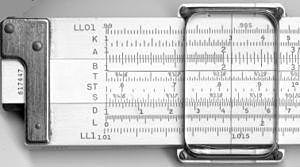
Imagine two identical rectangular pieces of wood (slats) sitting side by side. Each slat is identically inscribed along its length with lines (ticks) representing numerical values. The distance from the end of the slat to any particular tick x is log x. For example, the distance from the end of the slat to the tick labeled 8 is log 8. To multiply two numbers x and y, slide one of the slats so that its end is opposite x on the other slat. Under the tick for y on the sliding slat will be the tick for xy on the stationary slat.

Let’s call the two slats A and B. To multiply 3 x 5, you move slat A so that its end is positioned over 3 on stationary slat B. Now look at 5 on slat A. The number showing on slat B will be 15 (the product). To divide, you simply go the other way. For instance, to divide 15 by 3, move slat A in the other direction so that its end is positioned over 3 on the stationary slat B. Now look at 15 on slat A, the number showing on slat B will be 5.

So how does it work?

To repeat, the numbers shown on A and B are positioned from the end of the slats according to their logarithms. That is, the tick for any number y on slat B is at distance log x + log y = log xy from the end of slat A. In our example, log 3 + log 5 = log 3 x 5 = 15. Isn’t that clever?

The slide rule is not as precise as a Briggs table.  The best slide rules could get only three digits of accuracy, considerably less than in the tables, which in Briggs’ day had already been calculated to 14 digits of accuracy. Nevertheless, the slide rule is still extremely valuable because it trades speed for precision. Skilled slide-rule wielding users could do long chains of calculations very quickly and get three digits of precision in their answers.

Being able to multiply and divide mechanically would already be of considerable use, but slide rules can also be used to mechanically carry out numerous other mathematical operations. On my beloved Keuffel & Esser (once considered the Rolls Royce slide rules), there are in fact 20 scales for finding reciprocals, squares and square roots, multiplication by pi, trigonometric functions (sine, cosine, tangent, cotangent, secant, cosecant), etc.

The first practical slide rules were not simply two slats laid next to each other. Other configurations were tried, such as round and cylindrical. But since these were very hard to build in the 1600s, straight slide rules became the standard.

The basic configuration consisted of three slats of equal length bound to each other by clasps at the ends. The upper and lower slats were fixed by the claps, while the middle one slid back and forth between them. As in the examples above, to do a calculation you slid the middle slat to the appropriate position and then read the result on the appropriate scale above or below it. Given that there were several scales on the slat above and below the sliding slat, the slide came with a movable cursor to facilitate reading the result on the appropriate scale. 

It probably will not have escaped your notice (at least I hope it will not have escaped your notice) that adding and subtracting logarithms by moving slats back and forth are analog operations and thus inherently subject to error. This is indeed a drawback of the slide rule. There is also inherent inaccuracy in the algorithms used to calculate the original logarithms on which the slide rule is based. However, as noted above, this source of potential error is many orders of magnitude less important than the inaccuracy inherent in the analog movements of the slats of the device itself. 

Working with simple numbers most often gives precise answers, but with more complicated numbers some interpolation is required, hence a possible error. For example, multiplying integers (e.g. 2 x 3, 3 x 5, etc.) runs little risk of error because these numbers are clearly marked on the slide rule slats. However, 2.4 x 3.5 or 4.11 x 5.23 are not so clearly marked.

The standard length of a slide rule is 25 centimeters (approximately11 inches). The accuracy of the slide rule can be increased by increasing its length, say to 40 centimeters; however, this would be at the cost of portability. Certain people found even the standard 25-centimeter model too cumbersome, so manufacturers also offered models as short as 10 centimeters, at best accurate to only two digits of precision. These were considered to be toys.

As a student, when I was with my more geeky friends, I would clip my slide rule onto my belt. When I was with less geeky friends, I would hide it away in my briefcase or tote bag. Neither stratagem would have been feasible with a larger instrument.

Theoretically, with a standard slide rule, there were two possible solutions to the problem of accuracy.

1. Use the slide rule when small possible errors would be insignificant to the purpose of the calculation.
2. Do calculations by hand when possible errors inherent in the slide rule would be significant to the purpose of the calculation.

Lest we forget, it is not necessary for a slide rule to be straight. As noted earlier, pioneers in the 1600s already experimented (and failed) with building round and cylindrical instruments. With a round slide rule, aligning two logarithmic lengths occurs by turning a wheel rather than moving a slat. This makes the slide rule considerably more compact and easier to carry around. It has essentially the same accuracy as a straight slide rule; however, it is possible to manipulate the wheel in such a way as to increase the accuracy when really desired. The cylindrical slide rule is also more compact than the straight model with essentially the same accuracy.

From the 1600s and into the 1900s, gears-and-levels machines were developed that could rapidly do addition and subtraction, but could not do multiplication or division. Blaise Pascal invented such a machine around 1650. By contrast, the slide rule could rapidly do multiplication and division, but could not do addition and subtraction. It took until the 20th century to learn how to build mechanical calculators that did all four arithmetic operations. However, these were bulky, slow, expensive, and easily jammed. You certainly couldn’t put one of them on your belt or in your briefcase.

But no matter what the configuration, the problem of accuracy still remains. This was probably the prime reason the slide rule started to decline with the introduction of affordable pocket digital calculators in the 1970s. Being digital rather than analog (no scaling, direct numeric readout), these ingenious compact devices seemed destined to consign the slide rule to the dustbin of history literally almost overnight. However, it didn’t quite work out that way because digital calculators have their own inherent precision problems.

For example, Intel suffered a scandal in the 1990s because its way of handling floating point numbers conflicted with the way a spreadsheet calculated, leading to incorrect calculations on the spreadsheet. There were lawsuits from users whose businesses were negatively impacted by erroneous spreadsheet calculations.

As Peter Denning, Ubiquity’s editor and former user of Keuffel & Esser slide rules, puts it, “Rounding off error is always a problem in iterative algorithms, because the error can accumulate with each cycle of the algorithm. We may have buried errors a bit deeper with higher precision machines, but they are still there. Nevertheless, the HP-35 (1972) must be considered a breakthrough because it combined the arithmetical digital machine with the functional interface of the slide rule. On this device, you could do any slide rule function and get many more than 3 digits of precision. You could also handle complex arithmetic expressions. I could program it for simple algorithms that combined arithmetic and slide-rule function as their algorithm steps. All for $400—and of course considerably less today!”

Another advantage. With digital calculators, you can also add and subtract, but with a slide rule you can’t. In other words, with a slide rule you can solve a problem like 14 x 7 = 98, but you can’t solve a problem like 14 + 7 = 21. Well, actually, this isn’t entirely true. There is a rather complicated method for adding and subtracting on a slide rule, but you probably wouldn’t want to do it.

To the best of my knowledge, round slide rules are still being used in aviation. But this appears to be their last stand. In the foreseeable future, slide rules seem destined to become venerated museum pieces to those of us who actually used them, and just quaint historical relics for those who never did.

I mourn their passing.

---